Bestseller #2

- LRS Account Books Copy Size Combo – Hard Bound – 20 x 16 cm
- Ledger + Cash Book + Stock Copy + Attendance Copy
- Heavy Hard Bound to protect the pages efficiently ; Manually Stitched
₹499
Bestseller #3
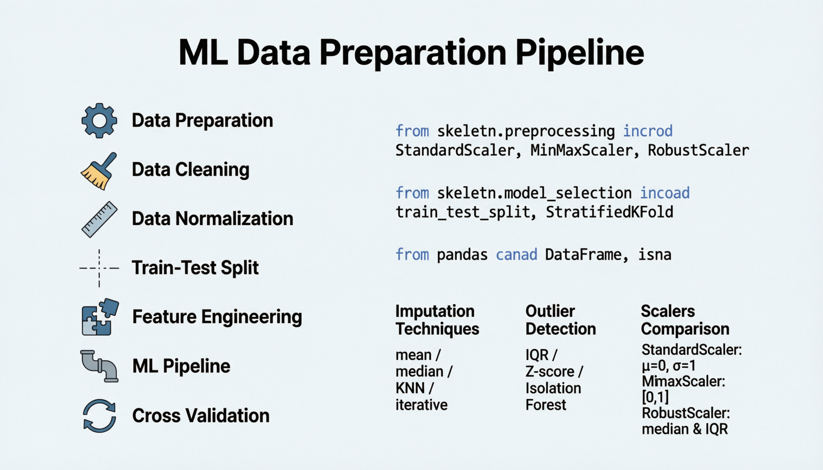
Step 3 of ML Pipeline
Data Preparation
Clean, Normalize, and Split Your Data
1 Data Cleaning
Remove or handle missing values, outliers, duplicates, and inconsistencies in your dataset to ensure data quality and model reliability.
🔍 Missing Values
Drop rows/columns or impute with mean, median, mode, or advanced methods
🎯 Outliers
Identify using IQR, Z-score, or domain knowledge; remove or cap extreme values
🔄 Duplicates
Remove exact or near-duplicate records that can bias your model
✅ Validation
Check data types, ranges, and format consistency across features
Example: Handling Missing Values and Outliers
import pandas as pd
import numpy as np
from sklearn.impute import SimpleImputer

# Load sample dataset
df = pd.DataFrame({
    'age': [25, 30, np.nan, 35, 40, 200, 28],
    'salary': [50000, 60000, 55000, np.nan, 70000, 65000, 52000],
    'city': ['NYC', 'LA', 'Chicago', 'NYC', 'LA', 'Chicago', 'NYC']
})

# 1. Check missing values
print("Missing values:\n", df.isnull().sum())

# 2. Handle missing values - Imputation
imputer = SimpleImputer(strategy='mean')
df[['age', 'salary']] = imputer.fit_transform(df[['age', 'salary']])

# 3. Remove outliers using IQR method
Q1 = df['age'].quantile(0.25)
Q3 = df['age'].quantile(0.75)
IQR = Q3 - Q1
lower_bound = Q1 - 1.5 * IQR
upper_bound = Q3 + 1.5 * IQR

df_clean = df[(df['age'] >= lower_bound) & (df['age'] <= upper_bound)]

# 4. Remove duplicates
df_clean = df_clean.drop_duplicates()

print("\nCleaned data shape:", df_clean.shape)
Output:
Missing values:
age       1
salary    1
city      0

Cleaned data shape: (6, 3)
2 Data Normalization
Scale features to a similar range to improve model convergence and performance. Essential for distance-based algorithms and neural networks.
Standardization
Z-score normalization: Mean = 0, Std = 1
z = (x - μ) / σ
Use when: Data follows normal distribution, for algorithms sensitive to feature scale (SVM, KNN, Neural Networks)
Min-Max Scaling
Range [0, 1]: Preserves relationships
x' = (x - min) / (max - min)
Use when: Need bounded values, for image processing, neural networks with bounded activations
Robust Scaling
Uses median and IQR: Resistant to outliers
x' = (x - median) / IQR
Use when: Data contains outliers that can’t be removed
Example: Applying Different Scaling Techniques
from sklearn.preprocessing import StandardScaler, MinMaxScaler, RobustScaler
import pandas as pd

# Sample dataset
df = pd.DataFrame({
    'feature1': [100, 200, 300, 400, 500],
    'feature2': [10, 20, 15, 25, 30],
    'feature3': [0.1, 0.5, 1.2, 2.3, 3.1]
})

# 1. Standardization (StandardScaler)
scaler_standard = StandardScaler()
df_standard = pd.DataFrame(
    scaler_standard.fit_transform(df),
    columns=[f'{col}_std' for col in df.columns]
)

# 2. Min-Max Scaling
scaler_minmax = MinMaxScaler()
df_minmax = pd.DataFrame(
    scaler_minmax.fit_transform(df),
    columns=[f'{col}_mm' for col in df.columns]
)

# 3. Robust Scaling
scaler_robust = RobustScaler()
df_robust = pd.DataFrame(
    scaler_robust.fit_transform(df),
    columns=[f'{col}_rb' for col in df.columns]
)

print("Original data:")
print(df.head())
print("\nStandardized:")
print(df_standard.head(2))
print("\nMin-Max Scaled:")
print(df_minmax.head(2))
⚡ Pro Tip
Always fit your scaler on training data only, then transform both training and test sets using the same fitted scaler to prevent data leakage!
3 Train-Test Split
Divide your dataset into separate training and testing sets to evaluate model performance on unseen data and prevent overfitting.
1
Training Set
60-80% of data
Used to train the model
Used to train the model
2
Validation Set
10-20% of data
Tune hyperparameters
Tune hyperparameters
3
Test Set
10-20% of data
Final evaluation
Final evaluation
Example: Splitting Data with Stratification
from sklearn.model_selection import train_test_split
import pandas as pd
import numpy as np

# Create sample dataset
np.random.seed(42)
X = pd.DataFrame({
    'feature1': np.random.randn(1000),
    'feature2': np.random.randn(1000),
    'feature3': np.random.randn(1000)
})
y = np.random.choice([0, 1], size=1000, p=[0.7, 0.3])

# 1. Simple train-test split (80-20)
X_train, X_test, y_train, y_test = train_test_split(
    X, y,
    test_size=0.2,
    random_state=42
)

print("Training set size:", X_train.shape)
print("Test set size:", X_test.shape)

# 2. Train-Validation-Test split
# First split: separate test set (80-20)
X_temp, X_test, y_temp, y_test = train_test_split(
    X, y,
    test_size=0.2,
    random_state=42
)

# Second split: separate validation from training (75-25 of temp = 60-20 overall)
X_train, X_val, y_train, y_val = train_test_split(
    X_temp, y_temp,
    test_size=0.25,
    random_state=42
)

print("\n=== Train-Val-Test Split ===")
print(f"Training: {X_train.shape[0]} samples ({X_train.shape[0]/len(X)*100:.1f}%)")
print(f"Validation: {X_val.shape[0]} samples ({X_val.shape[0]/len(X)*100:.1f}%)")
print(f"Test: {X_test.shape[0]} samples ({X_test.shape[0]/len(X)*100:.1f}%)")

# 3. Stratified split (maintains class distribution)
X_train_strat, X_test_strat, y_train_strat, y_test_strat = train_test_split(
    X, y,
    test_size=0.2,
    stratify=y,  # Maintains class proportions
    random_state=42
)

print("\n=== Class Distribution ===")
print(f"Original: {np.bincount(y) / len(y)}")
print(f"Train: {np.bincount(y_train_strat) / len(y_train_strat)}")
print(f"Test: {np.bincount(y_test_strat) / len(y_test_strat)}")
Output:
Training set size: (800, 3)
Test set size: (200, 3)

=== Train-Val-Test Split ===
Training: 600 samples (60.0%)
Validation: 200 samples (20.0%)
Test: 200 samples (20.0%)

=== Class Distribution ===
Original: [0.703 0.297]
Train: [0.7025 0.2975]
Test: [0.705 0.295]
4 Complete Pipeline Example
Putting it all together: a complete data preparation pipeline from raw data to model-ready splits.
import pandas as pd
import numpy as np
from sklearn.model_selection import train_test_split
from sklearn.preprocessing import StandardScaler
from sklearn.impute import SimpleImputer

# Load dataset (example with Titanic-like data)
df = pd.DataFrame({
    'Age': [22, 38, 26, 35, np.nan, 54, 2, 27, 14, 4],
    'Fare': [7.25, 71.28, 7.92, 53.1, 8.05, 51.86, 21.08, np.nan, 11.13, 16.7],
    'Pclass': [3, 1, 3, 1, 3, 1, 3, 3, 2, 3],
    'Survived': [0, 1, 1, 1, 0, 0, 0, 1, 1, 1]
})

print("=== STEP 1: Data Cleaning ===")
# Handle missing values
imputer = SimpleImputer(strategy='median')
df[['Age', 'Fare']] = imputer.fit_transform(df[['Age', 'Fare']])
print(f"Missing values after imputation: {df.isnull().sum().sum()}")

# Remove duplicates
df = df.drop_duplicates()
print(f"Dataset shape after cleaning: {df.shape}")

print("\n=== STEP 2: Feature Engineering ===")
# Separate features and target
X = df.drop('Survived', axis=1)
y = df['Survived']
print(f"Features: {X.columns.tolist()}")
print(f"Target: Survived (Classes: {y.unique()})")

print("\n=== STEP 3: Train-Test Split ===")
# Split data (80-20 with stratification)
X_train, X_test, y_train, y_test = train_test_split(
    X, y,
    test_size=0.2,
    stratify=y,
    random_state=42
)
print(f"Training set: {X_train.shape}")
print(f"Test set: {X_test.shape}")

print("\n=== STEP 4: Feature Scaling ===")
# Scale features (fit on training data only)
scaler = StandardScaler()
X_train_scaled = scaler.fit_transform(X_train)
X_test_scaled = scaler.transform(X_test)  # Use fitted scaler

print(f"Training data mean: {X_train_scaled.mean(axis=0)}")
print(f"Training data std: {X_train_scaled.std(axis=0)}")

print("\n=== Data Ready for Modeling! ===")
print(f"X_train_scaled shape: {X_train_scaled.shape}")
print(f"X_test_scaled shape: {X_test_scaled.shape}")
Output:
=== STEP 1: Data Cleaning ===
Missing values after imputation: 0
Dataset shape after cleaning: (10, 4)

=== STEP 2: Feature Engineering ===
Features: ['Age', 'Fare', 'Pclass']
Target: Survived (Classes: [0 1])

=== STEP 3: Train-Test Split ===
Training set: (8, 3)
Test set: (2, 3)

=== STEP 4: Feature Scaling ===
Training data mean: [-0.  0.  0.]
Training data std: [1. 1. 1.]

=== Data Ready for Modeling! ===
X_train_scaled shape: (8, 3)
X_test_scaled shape: (2, 3)
🎯 Best Practices Checklist
- Always explore data before cleaning (use
df.info(),df.describe()) - Fit preprocessing steps (scalers, imputers) on training data only
- Use stratified splitting for imbalanced datasets
- Document all preprocessing steps for reproducibility
- Consider cross-validation for small datasets
- Save your fitted scalers/imputers for deployment
📚 Quick Reference
Data Cleaning
df.dropna()SimpleImputer()df.drop_duplicates()
Scaling
StandardScaler()MinMaxScaler()RobustScaler()
Splitting
train_test_split()stratify=yrandom_state=42
Validation
KFold()StratifiedKFold()cross_val_score()
Bestseller #1

Bestseller #2
Bestseller #3

Bestseller #4