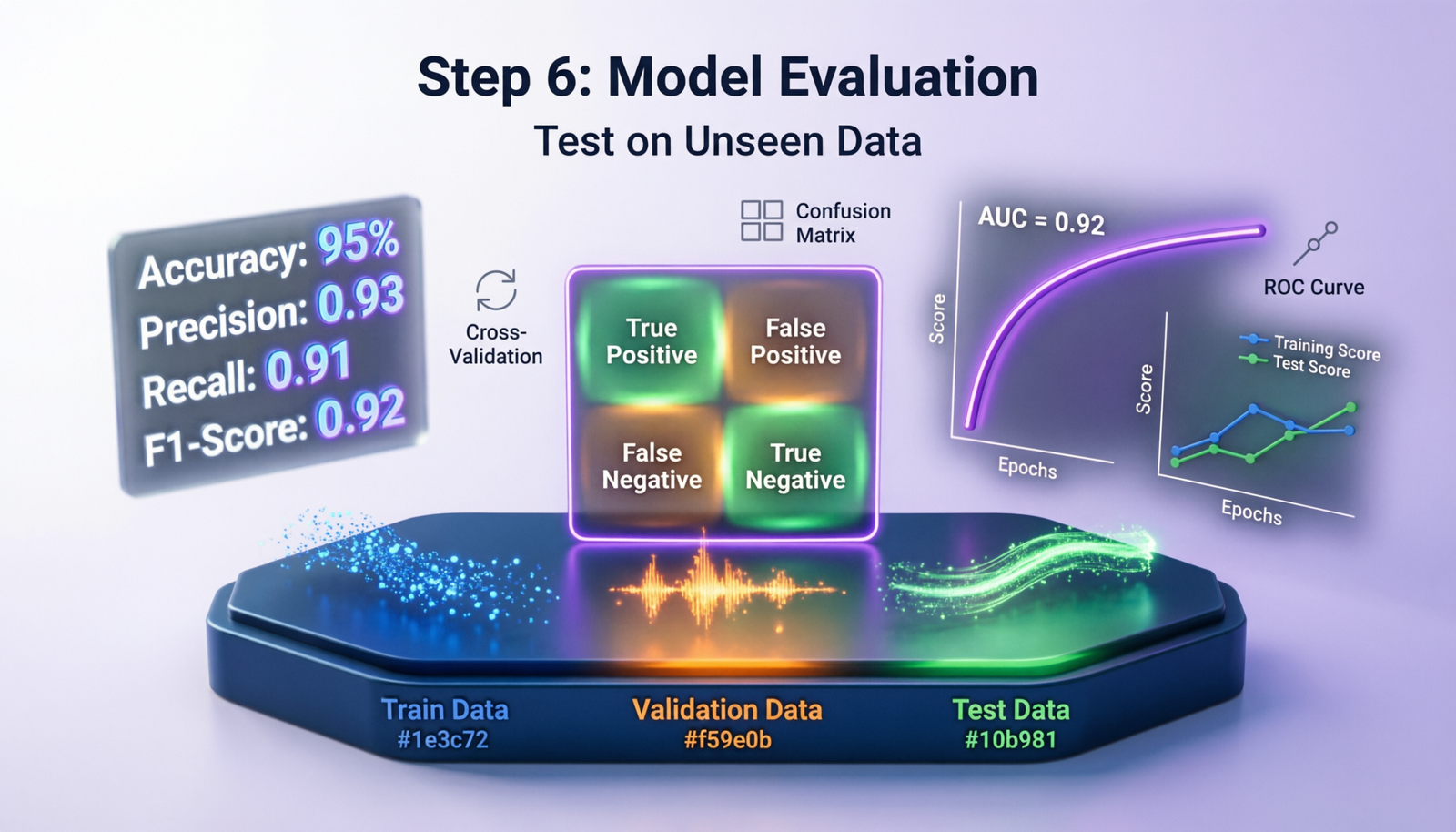
🎯Why Evaluate on Unseen Data?
Model evaluation on unseen data is crucial to assess how well your model generalizes to new, real-world scenarios. Training accuracy alone doesn’t guarantee good performance in production.
Key Principle: A model should perform well on data it has never seen during training. This tests its ability to generalize patterns rather than memorize training examples.
✂️Data Splitting Strategies
1. Train-Test Split
Simple division of data into training and testing sets
train_size = 70-80%
test_size = 20-30%
2. Train-Validation-Test Split
Three-way split for hyperparameter tuning
train = 60-70%
validation = 15-20%
test = 15-20%
3. K-Fold Cross-Validation
Multiple train-test splits for robust evaluation
k = 5 or 10 folds
Each fold serves as test set once
Example: Train-Test Split in Python
from sklearn.model_selection import train_test_split
X_train, X_test, y_train, y_test = train_test_split(
X, y,
test_size=0.2,
random_state=42,
stratify=y
)
print(f”Training samples: {len(X_train)}”)
print(f”Test samples: {len(X_test)}”)
Example: K-Fold Cross-Validation
from sklearn.model_selection import cross_val_score
from sklearn.ensemble import RandomForestClassifier
model = RandomForestClassifier()
scores = cross_val_score(model, X, y, cv=5)
print(f”Accuracy scores: {scores}”)
print(f”Mean accuracy: {scores.mean():.3f} (+/- {scores.std():.3f})”)
📈Classification Metrics
Confusion Matrix
Foundation for understanding classification performance:
| Actual \ Predicted |
Positive |
Negative |
| Positive |
True Positive (TP) |
False Negative (FN) |
| Negative |
False Positive (FP) |
True Negative (TN) |
Key Metrics
Accuracy
Accuracy = (TP + TN) / (TP + TN + FP + FN)
When to use: Balanced datasets
Precision
Precision = TP / (TP + FP)
When to use: Cost of false positives is high (e.g., spam detection)
Recall (Sensitivity)
Recall = TP / (TP + FN)
When to use: Cost of false negatives is high (e.g., disease detection)
F1-Score
F1 = 2 × (Precision × Recall) / (Precision + Recall)
When to use: Balance between precision and recall
Example: Classification Evaluation
from sklearn.metrics import classification_report, confusion_matrix
from sklearn.metrics import accuracy_score, precision_score, recall_score, f1_score
model.fit(X_train, y_train)
y_pred = model.predict(X_test)
accuracy = accuracy_score(y_test, y_pred)
precision = precision_score(y_test, y_pred, average=‘weighted’)
recall = recall_score(y_test, y_pred, average=‘weighted’)
f1 = f1_score(y_test, y_pred, average=‘weighted’)
print(f”Accuracy: {accuracy:.3f}”)
print(f”Precision: {precision:.3f}”)
print(f”Recall: {recall:.3f}”)
print(f”F1-Score: {f1:.3f}”)
print(“\nClassification Report:”)
print(classification_report(y_test, y_pred))
print(“\nConfusion Matrix:”)
print(confusion_matrix(y_test, y_pred))
ROC Curve & AUC
ROC-AUC Score: Measures the model’s ability to distinguish between classes
- AUC = 1.0: Perfect classifier
- AUC = 0.5: Random classifier
- AUC > 0.8: Good classifier
from sklearn.metrics import roc_auc_score, roc_curve
import matplotlib.pyplot as plt
y_proba = model.predict_proba(X_test)[:, 1]
auc_score = roc_auc_score(y_test, y_proba)
print(f”ROC-AUC Score: {auc_score:.3f}”)
fpr, tpr, thresholds = roc_curve(y_test, y_proba)
plt.plot(fpr, tpr, label=f’AUC = {auc_score:.3f}’)
plt.plot([0, 1], [0, 1], ‘k–‘)
plt.xlabel(‘False Positive Rate’)
plt.ylabel(‘True Positive Rate’)
plt.legend()
plt.show()
📉Regression Metrics
Mean Absolute Error (MAE)
MAE = (1/n) × Σ|y_true – y_pred|
Interpretation: Average absolute difference between predictions and actual values
Mean Squared Error (MSE)
MSE = (1/n) × Σ(y_true – y_pred)²
Interpretation: Penalizes larger errors more heavily
Root Mean Squared Error (RMSE)
RMSE = √MSE
Interpretation: Same units as target variable
R² Score (Coefficient of Determination)
R² = 1 – (SS_res / SS_tot)
Interpretation: Proportion of variance explained (0 to 1, higher is better)
Example: Regression Evaluation
from sklearn.metrics import mean_absolute_error, mean_squared_error, r2_score
import numpy as np
model.fit(X_train, y_train)
y_pred = model.predict(X_test)
mae = mean_absolute_error(y_test, y_pred)
mse = mean_squared_error(y_test, y_pred)
rmse = np.sqrt(mse)
r2 = r2_score(y_test, y_pred)
print(f”MAE: {mae:.3f}”)
print(f”MSE: {mse:.3f}”)
print(f”RMSE: {rmse:.3f}”)
print(f”R² Score: {r2:.3f}”)
plt.scatter(y_test, y_pred, alpha=0.5)
plt.plot([y_test.min(), y_test.max()],
[y_test.min(), y_test.max()], ‘r–‘)
plt.xlabel(‘Actual Values’)
plt.ylabel(‘Predicted Values’)
plt.title(f’R² = {r2:.3f}’)
plt.show()
⚠️Detecting Overfitting & Underfitting
| Scenario |
Training Performance |
Test Performance |
Issue |
| Good Fit |
High |
High (similar to train) |
✅ Model generalizes well |
| Overfitting |
Very High |
Low (much worse than train) |
❌ Model memorized training data |
| Underfitting |
Low |
Low |
❌ Model too simple |
Example: Learning Curves to Detect Overfitting
from sklearn.model_selection import learning_curve
train_sizes, train_scores, test_scores = learning_curve(
model, X, y,
cv=5,
train_sizes=np.linspace(0.1, 1.0, 10)
)
train_mean = np.mean(train_scores, axis=1)
train_std = np.std(train_scores, axis=1)
test_mean = np.mean(test_scores, axis=1)
test_std = np.std(test_scores, axis=1)
plt.plot(train_sizes, train_mean, label=‘Training score’)
plt.plot(train_sizes, test_mean, label=‘Cross-validation score’)
plt.fill_between(train_sizes, train_mean – train_std, train_mean + train_std, alpha=0.1)
plt.fill_between(train_sizes, test_mean – test_std, test_mean + test_std, alpha=0.1)
plt.xlabel(‘Training Examples’)
plt.ylabel(‘Score’)
plt.legend()
plt.show()
Warning Signs of Overfitting:
- Training accuracy >> Test accuracy (large gap)
- Training loss continues decreasing while validation loss increases
- Model performs perfectly on training data but poorly on new data
✨Best Practices for Model Evaluation
1. Never Use Test Data During Training
Test data should remain completely unseen until final evaluation. Using it during training or hyperparameter tuning leads to overoptimistic results.
2. Use Stratified Splitting for Imbalanced Data
Ensures each split maintains the same class distribution as the original dataset, preventing bias in evaluation.
3. Choose Metrics Based on Business Goals
Don’t rely solely on accuracy. Consider precision/recall for classification, and choose regression metrics that align with your use case.
4. Perform Cross-Validation for Small Datasets
K-fold cross-validation provides more reliable estimates when you have limited data, reducing the impact of how you split the data.
5. Monitor Both Training and Test Performance
Tracking both helps identify overfitting early. Use validation data during training to make decisions about when to stop.
🔄Complete Evaluation Pipeline Example
import pandas as pd
from sklearn.model_selection import train_test_split, cross_val_score
from sklearn.ensemble import RandomForestClassifier
from sklearn.metrics import classification_report, confusion_matrix, roc_auc_score
X = df.drop(‘target’, axis=1)
y = df[‘target’]
X_train, X_test, y_train, y_test = train_test_split(
X, y, test_size=0.2, random_state=42, stratify=y
)
model = RandomForestClassifier(n_estimators=100, random_state=42)
model.fit(X_train, y_train)
cv_scores = cross_val_score(model, X_train, y_train, cv=5)
print(f”Cross-validation scores: {cv_scores}”)
print(f”CV Mean: {cv_scores.mean():.3f} (+/- {cv_scores.std() * 2:.3f})”)
y_pred = model.predict(X_test)
y_proba = model.predict_proba(X_test)[:, 1]
print(“\nTest Set Performance:”)
print(classification_report(y_test, y_pred))
print(f”\nROC-AUC Score: {roc_auc_score(y_test, y_proba):.3f}”)
train_score = model.score(X_train, y_train)
test_score = model.score(X_test, y_test)
print(f”\nTraining Accuracy: {train_score:.3f}”)
print(f”Test Accuracy: {test_score:.3f}”)
print(f”Difference: {abs(train_score – test_score):.3f}”)
if abs(train_score – test_score) > 0.1:
print(“⚠️ Potential overfitting detected!”)
else:
print(“✅ Model generalizes well”)