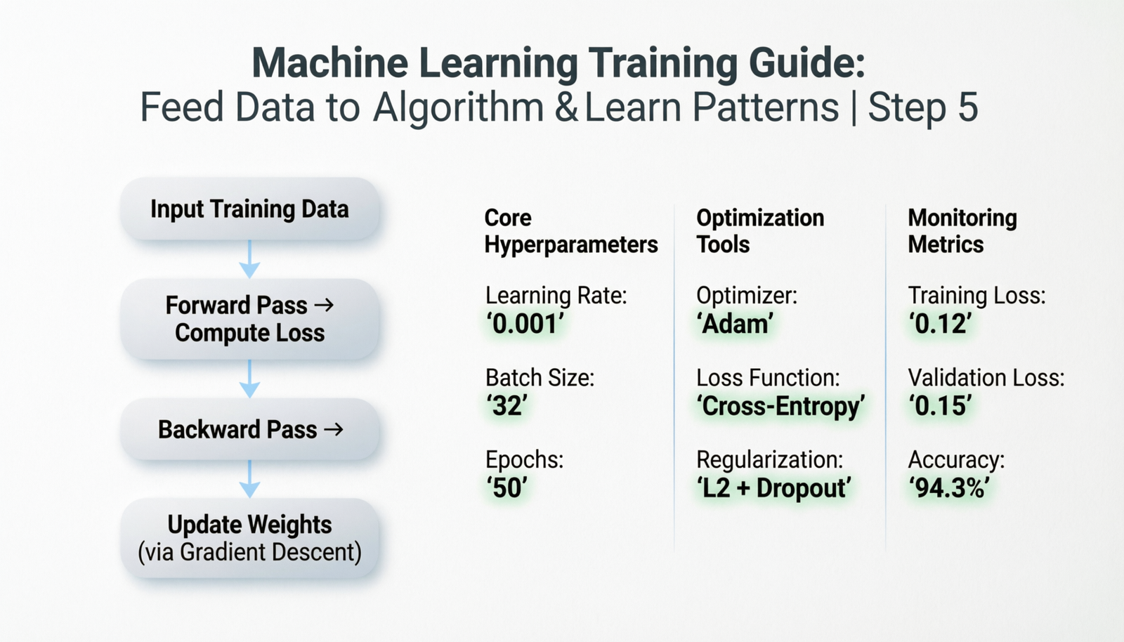
Step 5: Training
Feed Training Data to the Algorithm to Learn Patterns
What is Model Training?
Model training is the core process of machine learning where an algorithm learns patterns, relationships, and structures from training data. During this phase, the model adjusts its internal parameters to minimize the difference between its predictions and the actual outcomes in the training data. This iterative learning process enables the model to generalize from examples and make accurate predictions on new, unseen data.
Key Objective
The primary goal of training is to find the optimal set of parameters (weights and biases) that allow the model to accurately capture the underlying patterns in the data without overfitting to noise or memorizing specific examples.
The Training Process
1. Initialize Parameters
Set initial values for model weights and biases, typically using random initialization or pre-trained values.
2. Forward Pass
Feed training data through the model to generate predictions based on current parameters.
3. Calculate Loss
Compute the error between predictions and actual values using a loss function.
4. Backward Pass
Calculate gradients of the loss with respect to each parameter using backpropagation.
5. Update Parameters
Adjust weights and biases in the direction that reduces the loss using an optimization algorithm.
6. Iterate
Repeat steps 2-5 for multiple epochs until the model converges or meets stopping criteria.
Training Flow Diagram
Training Data
Initialize Model Parameters
Forward Pass → Generate Predictions
Calculate Loss Function
Backward Pass → Compute Gradients
Update Parameters (Optimization)
Check Convergence
Trained Model
Training for Different Algorithm Types
Supervised Learning
Process: Model learns from labeled examples by minimizing prediction error.
Examples:
- Linear/Logistic Regression
- Decision Trees
- Neural Networks
- Support Vector Machines
Unsupervised Learning
Process: Model discovers hidden patterns and structures without labels.
Examples:
- K-Means Clustering
- PCA
- Autoencoders
- DBSCAN
Reinforcement Learning
Process: Agent learns through trial and error by maximizing cumulative rewards.
Examples:
- Q-Learning
- Policy Gradients
- Actor-Critic
- Deep Q-Networks
Key Training Concepts
1. Loss Functions
Loss functions measure how well the model’s predictions match the actual values. The choice of loss function depends on the problem type:
| Loss Function | Use Case | Description |
|---|---|---|
| Mean Squared Error (MSE) | Regression | Measures average squared difference between predictions and actual values |
| Binary Cross-Entropy | Binary Classification | Measures difference between predicted and actual probabilities for two classes |
| Categorical Cross-Entropy | Multi-class Classification | Extends binary cross-entropy to multiple classes |
| Huber Loss | Robust Regression | Combines MSE and MAE, less sensitive to outliers |
2. Optimization Algorithms
Optimization algorithms determine how model parameters are updated to minimize the loss function:
Gradient Descent Variants:
- Batch Gradient Descent: Uses entire dataset for each update (slow but stable)
- Stochastic Gradient Descent (SGD): Uses single sample for each update (fast but noisy)
- Mini-batch Gradient Descent: Uses small batches (balanced approach)
Advanced Optimizers:
- Adam: Adaptive learning rates with momentum (most popular)
- RMSprop: Adapts learning rates based on recent gradients
- AdaGrad: Adjusts learning rates for each parameter
- Momentum: Accelerates convergence by accumulating gradients
3. Learning Rate
The learning rate controls how much parameters are adjusted during each update:
- Too High: Model may overshoot optimal values and fail to converge
- Too Low: Training becomes extremely slow and may get stuck in local minima
- Optimal: Requires experimentation; techniques like learning rate scheduling can help
4. Batch Size
The number of training examples used in one iteration:
- Small batches (8-32): More updates, faster convergence, higher noise, better generalization
- Large batches (256+): Fewer updates, more stable gradients, better hardware utilization
- Trade-off: Balance between computational efficiency and generalization
5. Epochs
One epoch represents a complete pass through the entire training dataset. Key considerations:
- Too Few Epochs: Underfitting – model hasn’t learned enough
- Too Many Epochs: Overfitting – model memorizes training data
- Early Stopping: Monitor validation loss and stop when it stops improving
Training Example: Neural Network
Monitoring Training Progress
Key Metrics to Track:
| Metric | What It Measures | What to Look For |
|---|---|---|
| Training Loss | Error on training data | Should steadily decrease |
| Validation Loss | Error on validation data | Should decrease and stabilize |
| Training Accuracy | Performance on training data | Should increase |
| Validation Accuracy | Performance on validation data | Should increase without large gap from training |
Common Training Patterns:
✅ Good Training:
- Both training and validation loss decrease together
- Small gap between training and validation metrics
- Smooth learning curves without large fluctuations
⚠️ Overfitting:
- Training loss continues decreasing but validation loss increases
- Large gap between training and validation accuracy
- Model performs well on training data but poorly on validation data
⚠️ Underfitting:
- Both training and validation loss remain high
- Model fails to capture patterns in the data
- Poor performance on both training and validation sets
Advanced Training Techniques
1. Regularization
Techniques to prevent overfitting by adding constraints to the model:
- L1 Regularization (Lasso): Adds absolute value of weights to loss (feature selection)
- L2 Regularization (Ridge): Adds squared weights to loss (weight decay)
- Elastic Net: Combines L1 and L2 regularization
- Dropout: Randomly deactivates neurons during training
2. Data Augmentation
Artificially expanding the training dataset by creating modified versions of existing data:
- Image transformations (rotation, flipping, cropping, color adjustment)
- Text augmentation (synonym replacement, back-translation)
- Time series jittering and scaling
3. Transfer Learning
Using pre-trained models as a starting point:
- Leverage knowledge from models trained on large datasets
- Fine-tune on specific task with less data
- Faster training and better performance
4. Learning Rate Scheduling
Adjusting the learning rate during training:
- Step Decay: Reduce learning rate at fixed intervals
- Exponential Decay: Gradually decrease learning rate
- Cosine Annealing: Cyclical learning rate schedule
- Adaptive: Reduce when validation loss plateaus
5. Batch Normalization
Normalize inputs to each layer to stabilize and accelerate training:
- Reduces internal covariate shift
- Allows higher learning rates
- Provides some regularization effect
Training Best Practices
✓ Recommended Practices:
- Start Simple: Begin with a baseline model before adding complexity
- Split Your Data: Use separate train, validation, and test sets
- Monitor Everything: Track multiple metrics during training
- Use Cross-Validation: Especially with limited data
- Implement Early Stopping: Prevent wasting time on overfitting
- Save Checkpoints: Regularly save model states during training
- Experiment Systematically: Change one hyperparameter at a time
- Normalize Inputs: Scale features to similar ranges
- Handle Class Imbalance: Use appropriate sampling or weighting techniques
- Validate Thoroughly: Ensure model generalizes to unseen data
Common Training Challenges
1. Vanishing/Exploding Gradients
Problem: Gradients become too small or too large in deep networks
Solutions:
- Use appropriate activation functions (ReLU, LeakyReLU)
- Implement batch normalization
- Use gradient clipping
- Apply proper weight initialization
2. Slow Convergence
Problem: Model takes too long to train
Solutions:
- Increase learning rate (carefully)
- Use advanced optimizers (Adam, RMSprop)
- Implement learning rate warm-up
- Add batch normalization
3. Mode Collapse (GANs)
Problem: Generator produces limited variety of outputs
Solutions:
- Adjust learning rates for generator and discriminator
- Use different loss functions
- Implement mini-batch discrimination
4. Catastrophic Forgetting
Problem: Model forgets previously learned information when learning new tasks
Solutions:
- Implement elastic weight consolidation
- Use progressive neural networks
- Apply memory replay techniques
Hardware Considerations
Training Infrastructure:
| Hardware | Best For | Considerations |
|---|---|---|
| CPU | Small models, traditional ML algorithms | Slower for deep learning, more accessible |
| GPU | Deep learning, computer vision, large models | Parallel processing, requires CUDA/cuDNN |
| TPU | Very large models, production deployment | Optimized for TensorFlow, cloud-based |
| Distributed Training | Massive datasets, huge models | Requires special frameworks, complex setup |
Mixed Precision Training:
Using lower precision (16-bit instead of 32-bit) to speed up training:
- Reduces memory usage (can train larger models)
- Faster computation on modern GPUs
- Minimal impact on model accuracy
- Enables training of bigger batch sizes
Summary
Key Takeaways:
- Training is an iterative process where models learn patterns from data by adjusting parameters
- The training process involves forward passes, loss calculation, backpropagation, and parameter updates
- Success depends on proper hyperparameter tuning (learning rate, batch size, epochs)
- Monitor both training and validation metrics to detect overfitting or underfitting
- Advanced techniques like regularization, data augmentation, and transfer learning improve performance
- Different algorithms require different training approaches and considerations
- Hardware choice significantly impacts training speed and feasibility
The training phase is where machine learning models develop their predictive capabilities. By carefully managing the training process, monitoring progress, and applying appropriate techniques, you can develop robust models that generalize well to new data. Remember that training is both an art and a science, requiring experimentation, patience, and continuous refinement to achieve optimal results.