Recurrent Neural Networks (RNNs) — Complete Guide with Examples
Deep Learning Series | A comprehensive guide to RNNs with code examples.
Table of Contents
- What is an RNN?
- How RNNs Work
- Types of RNNs
- LSTM & GRU
- Code Example: NumPy from Scratch
- Code Example: PyTorch LSTM
- Code Example: Keras GRU
- Code Example: Sentiment Analysis
- Common Problems & Solutions
- Real-World Applications
- RNN vs CNN vs FNN
- Summary
1. What is a Recurrent Neural Network?
A Recurrent Neural Network (RNN) is a type of artificial neural network designed to work with sequential or time-series data. Unlike feedforward networks that process inputs independently, RNNs have a memory mechanism — they retain information from previous steps and use it to influence future outputs.
Think of reading a sentence: understanding the word “bank” depends on whether you read “river bank” or “bank account.” RNNs solve this by maintaining a hidden state that carries context through each time step.
Key Intuition: The defining feature of an RNN is that its outputs are fed back as inputs to the next step. This creates a loop — a form of short-term memory that allows the network to process sequences of arbitrary length.
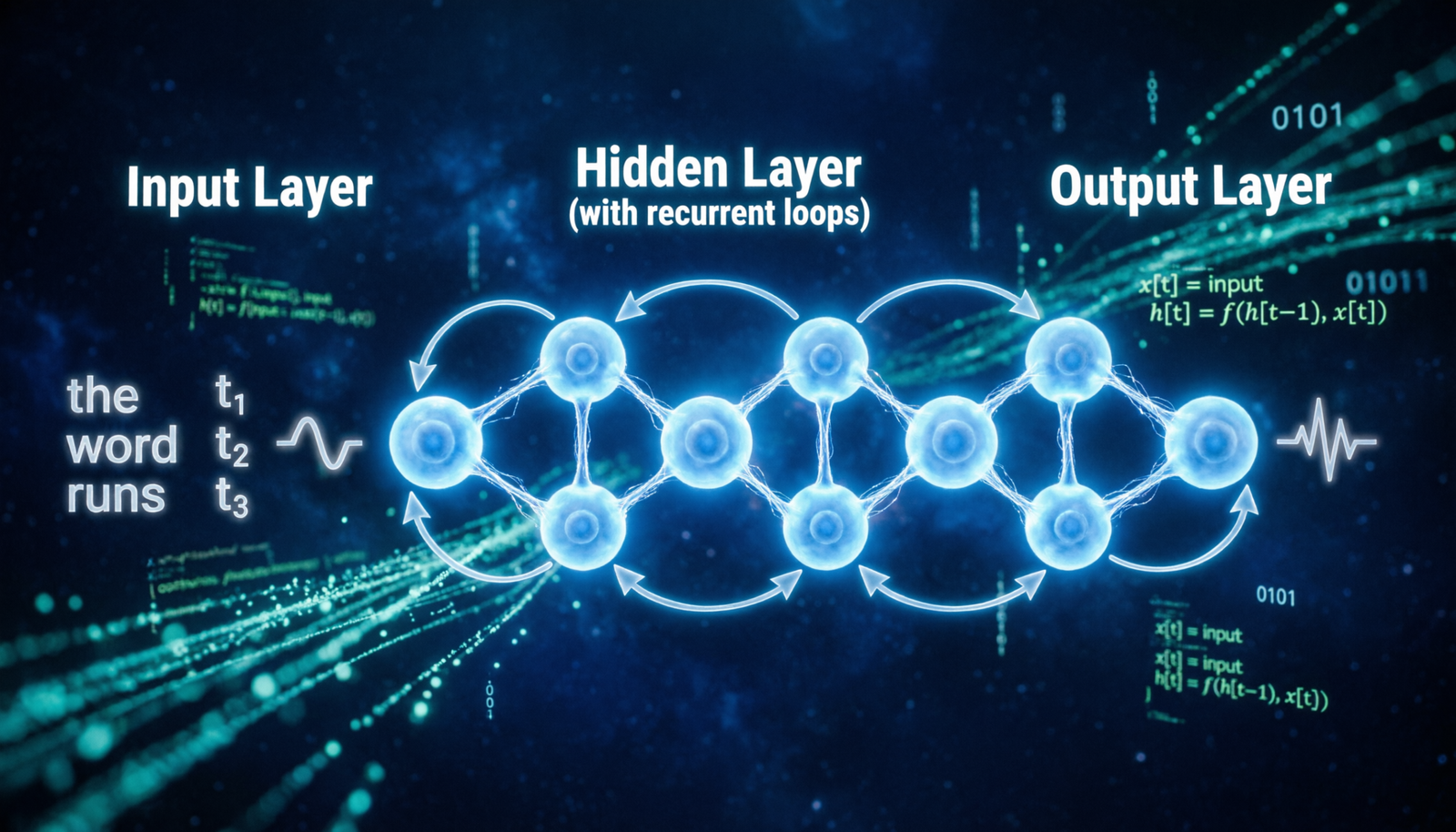
2. How RNNs Work
At each time step t, an RNN takes two inputs: the current input x_t and the previous hidden state h_(t-1). It produces a new hidden state h_t and optionally an output y_t.
Unrolled RNN Diagram
         y0          y1          y2          y3
         |           |           |           |
    +---------+  +---------+  +---------+  +---------+
    |   h0    |->|   h1    |->|   h2    |->|   h3    |
    +---------+  +---------+  +---------+  +---------+
      ^  |          ^              ^              ^
      |  +--loop    |              |              |
         x0         x1            x2             x3

  Each node shares the same weights W, U, V across all time steps.
  The loop arrow represents the recurrent connection (memory).
Core Equations
  // Hidden state update
  h_t = tanh(W_h * h_(t-1) + W_x * x_t + b_h)

  // Output calculation
  y_t = W_y * h_t + b_y

  Where:
    W_h = weight matrix for hidden state
    W_x = weight matrix for input
    W_y = weight matrix for output
    b_h, b_y = bias vectors
    tanh = hyperbolic tangent activation function
3. Types of RNN Architectures
RNNs come in several configurations depending on the relationship between inputs and outputs:
| Architecture | Description | Example Use Case |
|---|---|---|
| One-to-One | Single input → Single output. Standard neural network. | Image classification |
| One-to-Many | Single input → Sequence output. | Image captioning |
| Many-to-One | Sequence input → Single output. | Sentiment analysis |
| Many-to-Many (sync) | Sequence input → Sequence output (same length). | POS tagging |
| Many-to-Many (async) | Encoder-decoder. Sequence in → Sequence out (different length). | Machine translation |
| Bidirectional | Processes sequence forward AND backward. | Named entity recognition |
4. LSTM & GRU
Vanilla RNNs struggle with long sequences due to the vanishing gradient problem. Two architectures solve this with learned gating mechanisms:
LSTM — Long Short-Term Memory
LSTMs introduce a cell state (long-term memory) alongside the hidden state (short-term memory). Three learned gates control information flow:
  // Forget gate - what to erase from cell state
  f_t = sigmoid(W_f * [h_(t-1), x_t] + b_f)

  // Input gate - what new info to store
  i_t = sigmoid(W_i * [h_(t-1), x_t] + b_i)
  C_tilde = tanh(W_C * [h_(t-1), x_t] + b_C)

  // Cell state update
  C_t = f_t * C_(t-1) + i_t * C_tilde

  // Output gate
  o_t = sigmoid(W_o * [h_(t-1), x_t] + b_o)
  h_t = o_t * tanh(C_t)
GRU — Gated Recurrent Unit
GRUs merge the forget and input gates into a single update gate and combine the cell and hidden states. Fewer parameters, often comparable performance to LSTM:
  // Reset gate - how much past to forget
  r_t = sigmoid(W_r * [h_(t-1), x_t])

  // Update gate - how much past to keep
  z_t = sigmoid(W_z * [h_(t-1), x_t])

  // Candidate hidden state
  h_tilde = tanh(W * [r_t * h_(t-1), x_t])

  // Final hidden state
  h_t = (1 - z_t) * h_(t-1) + z_t * h_tilde
5. Code Example: Simple RNN from Scratch (NumPy)
A minimal RNN built from scratch using only NumPy to understand the core mechanics:
import numpy as np

# --- Minimal RNN from scratch ---

class SimpleRNN:
    def __init__(self, input_size, hidden_size, output_size):
        # Xavier initialization
        self.W_xh = np.random.randn(hidden_size, input_size) * 0.01
        self.W_hh = np.random.randn(hidden_size, hidden_size) * 0.01
        self.W_hy = np.random.randn(output_size, hidden_size) * 0.01
        self.b_h  = np.zeros((hidden_size, 1))
        self.b_y  = np.zeros((output_size, 1))

    def forward(self, inputs):
        """
        inputs: list of one-hot encoded vectors (each shape: input_size x 1)
        Returns outputs and hidden states at each time step
        """
        h = np.zeros((self.W_hh.shape[0], 1))  # initial hidden state
        outputs, hidden_states = [], [h]

        for x in inputs:
            # Hidden state: h_t = tanh(W_xh*x + W_hh*h_prev + b_h)
            h = np.tanh(self.W_xh @ x + self.W_hh @ h + self.b_h)

            # Output: y_t = W_hy*h_t + b_y
            y = self.W_hy @ h + self.b_y

            outputs.append(y)
            hidden_states.append(h)

        return outputs, hidden_states


# --- Example: Process a 3-word sequence ---
input_size  = 4   # vocabulary size
hidden_size = 8   # hidden units
output_size = 4   # output size

rnn = SimpleRNN(input_size, hidden_size, output_size)

# Simulate 3 one-hot vectors (3 time steps)
sequence = [
    np.array([[1], [0], [0], [0]]),   # word "hello"
    np.array([[0], [1], [0], [0]]),   # word "world"
    np.array([[0], [0], [1], [0]]),   # word "rnn"
]

outputs, hidden_states = rnn.forward(sequence)
print(f"Outputs per step: {[o.shape for o in outputs]}")
print(f"Hidden states:    {len(hidden_states)} of shape {hidden_states[0].shape}")
6. Code Example: LSTM Classifier (PyTorch)
Using PyTorch’s built-in LSTM module for text classification:
import torch
import torch.nn as nn

# --- Bidirectional LSTM Text Classifier ---

class LSTMClassifier(nn.Module):
    def __init__(self, vocab_size, embed_dim, hidden_dim, num_classes, n_layers=2):
        super(LSTMClassifier, self).__init__()

        # Embedding: token indices -> dense vectors
        self.embedding = nn.Embedding(vocab_size, embed_dim, padding_idx=0)

        # Bidirectional LSTM with dropout
        self.lstm = nn.LSTM(
            input_size=embed_dim,
            hidden_size=hidden_dim,
            num_layers=n_layers,
            batch_first=True,
            bidirectional=True,
            dropout=0.3
        )

        self.dropout = nn.Dropout(0.3)
        self.fc = nn.Linear(hidden_dim * 2, num_classes)  # *2 for bidirectional

    def forward(self, x):
        embedded = self.dropout(self.embedding(x))
        output, (hidden, cell) = self.lstm(embedded)

        # Concatenate final forward + backward hidden states
        hidden = torch.cat((hidden[-2], hidden[-1]), dim=1)
        hidden = self.dropout(hidden)
        return self.fc(hidden)


# --- Setup ---
model = LSTMClassifier(
    vocab_size=10000,
    embed_dim=128,
    hidden_dim=256,
    num_classes=2       # positive / negative
)

optimizer = torch.optim.Adam(model.parameters(), lr=1e-3)
criterion = nn.CrossEntropyLoss()

def train_step(batch_x, batch_y):
    model.train()
    optimizer.zero_grad()
    predictions = model(batch_x)
    loss = criterion(predictions, batch_y)
    loss.backward()
    # Clip gradients to prevent exploding gradients
    nn.utils.clip_grad_norm_(model.parameters(), max_norm=1.0)
    optimizer.step()
    return loss.item()
7. Code Example: GRU Time-Series Predictor (Keras)
Using Keras/TensorFlow to build a stacked GRU model for time-series forecasting:
import tensorflow as tf
from tensorflow import keras
from tensorflow.keras import layers

# --- Stacked GRU for Time-Series Prediction ---

def build_gru_model(seq_len, n_features, n_units=64):
    model = keras.Sequential([
        layers.Input(shape=(seq_len, n_features)),

        # First GRU layer - return sequences for stacking
        layers.GRU(n_units, return_sequences=True, dropout=0.2),

        # Second GRU layer
        layers.GRU(n_units // 2, return_sequences=False),

        # Dense output
        layers.Dense(32, activation='relu'),
        layers.Dropout(0.2),
        layers.Dense(1)     # regression output
    ])
    return model


model = build_gru_model(seq_len=30, n_features=5)
model.compile(
    optimizer=keras.optimizers.Adam(learning_rate=0.001),
    loss='mse',
    metrics=['mae']
)

model.summary()

# Training with callbacks
history = model.fit(
    X_train, y_train,
    epochs=50,
    batch_size=32,
    validation_split=0.2,
    callbacks=[
        keras.callbacks.EarlyStopping(patience=5, restore_best_weights=True),
        keras.callbacks.ReduceLROnPlateau(factor=0.5, patience=3)
    ]
)
8. Code Example: Sentiment Analysis on IMDB (Keras)
Complete end-to-end sentiment analysis using a Bidirectional LSTM on the IMDB dataset:
from tensorflow.keras.datasets import imdb
from tensorflow.keras.preprocessing import sequence
from tensorflow.keras import layers, models

# --- Sentiment Analysis on IMDB Reviews ---

MAX_FEATURES = 10000   # vocabulary size
MAX_LEN      = 200     # max review length
EMBED_DIM    = 64

# Load pre-tokenized dataset
(X_train, y_train), (X_test, y_test) = imdb.load_data(num_words=MAX_FEATURES)

# Pad sequences to the same length
X_train = sequence.pad_sequences(X_train, maxlen=MAX_LEN)
X_test  = sequence.pad_sequences(X_test,  maxlen=MAX_LEN)

# Build Bidirectional LSTM model
model = models.Sequential([
    layers.Embedding(MAX_FEATURES, EMBED_DIM, mask_zero=True),
    layers.Bidirectional(layers.LSTM(64, return_sequences=True)),
    layers.Bidirectional(layers.LSTM(32)),
    layers.Dense(64, activation='relu'),
    layers.Dropout(0.5),
    layers.Dense(1, activation='sigmoid')   # binary: positive/negative
])

model.compile(
    optimizer='adam',
    loss='binary_crossentropy',
    metrics=['accuracy']
)

# Train
model.fit(X_train, y_train, epochs=5, batch_size=64, validation_split=0.2)

# Evaluate - typically achieves ~89-91% accuracy
loss, acc = model.evaluate(X_test, y_test)
print(f"Test Accuracy: {acc:.2%}")


# --- Predict on a new review ---
import numpy as np

word_index = imdb.get_word_index()

def encode_review(text):
    tokens = text.lower().split()
    encoded = [word_index.get(w, 2) + 3 for w in tokens]
    return sequence.pad_sequences([encoded], maxlen=MAX_LEN)

review = "This movie was absolutely fantastic and I loved every minute of it"
pred = model.predict(encode_review(review))[0][0]
print(f"Sentiment: {'Positive' if pred > 0.5 else 'Negative'} ({pred:.2%})")
9. Common Problems & Solutions
Problem 1: Vanishing Gradient
During backpropagation through time (BPTT), gradients are multiplied repeatedly. If weights are less than 1, gradients shrink exponentially toward zero — the network forgets distant past information and learning stalls for long sequences.
Solutions: Use LSTM or GRU gates • Use gradient clipping • Use residual connections
Problem 2: Exploding Gradient
The opposite of vanishing — if weights are greater than 1, gradients grow exponentially during BPTT, causing NaN values and unstable training. Common with deep or long RNNs.
Solutions: Gradient clipping (clip_grad_norm_) • Careful weight initialization
Problem 3: Long-Term Dependencies
Even with LSTM, very long sequences (500+ steps) can be hard to model. The network may fail to connect distant but relevant parts of a sequence (e.g., beginning of a paragraph to the end).
Solutions: Attention mechanisms • Transformer architecture
Problem 4: Slow Sequential Training
RNNs process time steps one by one — they cannot be parallelized like CNNs or Transformers. This makes training on very long sequences extremely slow on modern GPU hardware.
Solutions: Truncated BPTT • Move to Transformer-based models
10. Real-World Applications
- Speech Recognition — Converting audio waveforms to text (e.g., Siri, Google Assistant)
- Machine Translation — Translating between languages (e.g., early Google Translate)
- Sentiment Analysis — Classifying reviews as positive or negative
- Text Generation — Generating new text in a learned style
- Stock Price Forecasting — Predicting future prices from historical time series
- Music Generation — Composing melodies note by note
- Medical Diagnosis — Analyzing EHR sequences and patient timelines
- Chatbots & NLP — Understanding conversational context
- Image Captioning — Generating text descriptions from images
- Anomaly Detection — Spotting irregularities in logs or sensor data
11. RNN vs CNN vs Feedforward Neural Network
| Feature | RNN / LSTM / GRU | CNN | Feedforward (FNN / MLP) |
|---|---|---|---|
| Best For | Sequential / time-series data | Spatial data (images, video) | Tabular / fixed-size data |
| Memory | Hidden state (short & long term) | None between samples | None between samples |
| Input Size | Variable length sequences | Fixed spatial dimensions | Fixed vector size |
| Parallelizable | Limited (sequential steps) | Highly parallelizable | Fully parallelizable |
| Training Speed | Slow for long sequences | Fast with GPU | Very fast |
| Key Strength | Temporal patterns, NLP | Feature hierarchies, vision | Simple classification/regression |
| Popular Variants | LSTM, GRU, BiRNN, Seq2Seq | ResNet, VGG, EfficientNet | MLP, AutoEncoder |
| Handles Sequences? | Yes (natively) | Partially (with 1D conv) | No (fixed input only) |
12. Summary
- RNNs have memory. The hidden state carries information from previous time steps, enabling sequential data processing impossible for standard feedforward networks.
- LSTM & GRU solve vanishing gradients. Gating mechanisms selectively remember or forget information, enabling networks to learn both short and long-range dependencies.
- Many architecture variants exist. One-to-many, many-to-one, many-to-many, and bidirectional configurations cover virtually every sequential modeling scenario.
- Transformers are the modern successor. For most NLP tasks today, Transformer-based models (BERT, GPT) outperform RNNs due to better parallelism and attention mechanisms. However, RNNs remain valuable for streaming data and resource-constrained environments.
- Key hyperparameters to tune: hidden size, number of layers, dropout rate, learning rate, sequence length, and batch size.
Recurrent Neural Networks — Deep Learning Guide | RNN • LSTM • GRU • BiRNN