Building the Data Ingestion & Vector Indexing Layer
A complete guide to architecting high-throughput pipelines that transform raw documents into semantically searchable vector stores — the foundation of every production RAG system.
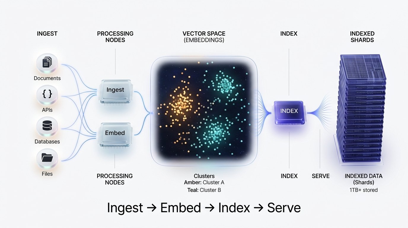
End-to-End Pipeline
The ingestion-to-retrieval pipeline consists of five major stages, each with distinct scaling characteristics and failure modes.
Data Ingestion Layer
The ingestion stage is responsible for connecting to heterogeneous data sources, pulling raw content, and normalising it into a consistent intermediate format before passing downstream. This layer must handle fault tolerance, deduplication, and incremental updates.
Document Loaders
PDFs via PyMuPDF, HTML via BeautifulSoup, DOCX via python-docx, and Markdown natively. Handle encoding normalisation early.
Database Connectors
SQL row serialisation, MongoDB document projection, and REST API pagination with exponential back-off retry logic.
Change Data Capture
Debezium-based CDC for real-time streaming. Kafka topics buffer updates before the embedding workers consume them.
Object Storage
S3 / GCS bucket watchers with event-driven triggers via SQS or Pub/Sub. Hash-based deduplication at this layer.
Connector Implementation (Python)
# Resilient document loader with retry + dedup
from langchain.document_loaders import UnstructuredPDFLoader
import hashlib, redis

dedup_store = redis.Redis(host="localhost", decode_responses=True)

def load_document(path: str) -> list:
    doc_hash = hashlib.sha256(open(path, "rb").read()).hexdigest()
    if dedup_store.exists(doc_hash):
        return []  # Already indexed — skip

    loader = UnstructuredPDFLoader(path, mode="elements")
    docs = loader.load()
    dedup_store.set(doc_hash, 1, ex=86400 * 30)  # 30-day TTL
return docsAlways attach source_url, ingested_at, doc_type, and tenant_id at ingestion time. Retrofitting metadata post-indexing requires a full re-index.
Chunking Strategy
Chunk size is the single most impactful parameter in any RAG system. Too small and you lose context; too large and you dilute relevance. The goal is semantically coherent units that embed into tight, discriminable vectors.
| Strategy | Chunk Size | Best For | Coherence | Speed |
|---|---|---|---|---|
| Fixed-size | 512 tokens | Homogeneous corpora | Medium | Fast |
| Recursive Character | 500–1000 tok | Mixed-format docs | High | Fast |
| Semantic / Sentence | Variable | Dense technical text | Very High | Moderate |
| Document-aware | Section-level | Structured reports | Highest | Slow |
| Small-to-big | 128 + 512 tok | Multi-granularity RAG | High | Moderate |
Recursive Splitter with Overlap
from langchain.text_splitter import RecursiveCharacterTextSplitter

splitter = RecursiveCharacterTextSplitter(
    chunk_size=600,
    chunk_overlap=80,       # ~13% overlap preserves boundary context
    separators=["\n\n", "\n", ".", " ", ""],
    length_function=tiktoken_len,  # Token-accurate, not char-based
    add_start_index=True
)

chunks = splitter.split_documents(docs)
# Propagate parent metadata to each chunk
for chunk in chunks:
    chunk.metadata["chunk_id"] = uuid4().hex()
chunk.metadata["token_count"] = tiktoken_len(chunk.page_content)Index child chunks (128 tokens) for precision retrieval, but return the parent chunk (512 tokens) to the LLM. This dramatically improves both recall and generation quality.
Embedding Generation
The embedding model maps each text chunk to a high-dimensional dense vector. The choice of model directly determines the semantic quality of your retrieval and should be matched to your domain and language.
Batch Construction
Group chunks into batches of 100–2048 based on API limits. Sort by token length to minimise padding waste in batch-encode mode.
Rate-Limited API Calls
Use asyncio with a semaphore to cap concurrent requests. Implement token-bucket rate limiting against the provider’s TPM limits.
Normalisation
L2-normalise all vectors before storage. Normalised cosine similarity becomes a simple dot product — dramatically faster in the vector DB.
Caching Layer
Cache embeddings keyed by chunk hash in Redis or a local SQLite store. On re-ingestion of unchanged documents, skip the API call entirely.
Async Batch Embedding Worker
import asyncio, numpy as np
from openai import AsyncOpenAI

client = AsyncOpenAI()
SEMAPHORE = asyncio.Semaphore(10)  # Max 10 concurrent requests

async def embed_batch(texts: list[str]) -> np.ndarray:
    async with SEMAPHORE:
        resp = await client.embeddings.create(
            model="text-embedding-3-small",
            input=texts
        )
    vecs = np.array([d.embedding for d in resp.data], dtype="float32")
    return vecs / np.linalg.norm(vecs, axis=1, keepdims=True)  # L2-norm

async def embed_all(chunks: list, batch_size=256):
    tasks = [embed_batch(chunks[i:i+batch_size])
              for i in range(0, len(chunks), batch_size)]
return np.vstack(await asyncio.gather(*tasks))Vector Index Construction
The vector index is the search engine of your RAG system. It trades index build time and memory for query-time speed. The dominant algorithm for production is HNSW — a graph-based approximate nearest-neighbour structure.
HNSW
Hierarchical Navigable Small World. O(log n) queries. Best recall/speed trade-off. High memory usage (~300 bytes/vector).
IVF-Flat
Inverted File Index with flat quantization. Low memory, slower build. Good for multi-tenant workloads with namespace-level isolation.
IVF-PQ
Product Quantization compresses vectors 8–32×. Ideal for billion-scale corpora where memory is the binding constraint.
DiskANN
Graph-based index on SSD storage. Enables sub-50ms queries on 1B+ vector datasets with a fraction of HNSW’s RAM cost.
Qdrant Upsert with Payload Filtering
from qdrant_client import QdrantClient, models

qdrant = QdrantClient(url="http://localhost:6333")

qdrant.recreate_collection(
    collection_name="knowledge_base",
    vectors_config=models.VectorParams(
        size=1536, distance=models.Distance.COSINE
    ),
    hnsw_config=models.HnswConfigDiff(
        m=16,            # Edges per node — higher = better recall
        ef_construct=200  # Build-time beam width
    )
)

# Batch upsert with metadata payload
qdrant.upsert(
    collection_name="knowledge_base",
    points=[
        models.PointStruct(
            id=chunk.metadata["chunk_id"],
            vector=embedding.tolist(),
            payload={
                "text": chunk.page_content,
                "source": chunk.metadata["source"],
                "tenant_id": chunk.metadata["tenant_id"],
                "doc_type": chunk.metadata["doc_type"],
            }
        )
        for chunk, embedding in zip(chunks, embeddings)
    ]
)Increasing m from 16 to 32 boosts recall@10 by ~3% but doubles memory. Profile on your actual data distribution before setting production HNSW params.
Query & Retrieval Flow
At query time, the user’s question is embedded using the same model used during indexing, then an ANN search finds the top-k most similar chunks. Hybrid retrieval (dense + sparse BM25) consistently outperforms vector-only search.
Hybrid Retrieval with Re-Ranking
from qdrant_client import models
from cohere import Client as Cohere

co = Cohere()

async def retrieve(query: str, tenant_id: str, top_k=20):
    q_vec = (await embed_batch([query]))[0]

    # Filtered ANN search (tenant isolation)
    hits = qdrant.search(
        collection_name="knowledge_base",
        query_vector=q_vec.tolist(),
        query_filter=models.Filter(
            must=[models.FieldCondition(
                key="tenant_id",
                match=models.MatchValue(value=tenant_id)
            )]
        ),
        limit=top_k,
        with_payload=True
    )

    # Cohere rerank for precision
    docs = [h.payload["text"] for h in hits]
    ranked = co.rerank(query=query, documents=docs, top_n=5)
return [docs[r.index] for r in ranked.results]Best Practices & Architecture
Running a vector indexing layer in production requires careful attention to observability, cost, and operational hygiene. The following principles are derived from large-scale deployments.
Version your embedding model
Store the model name and version in every chunk’s metadata. When you upgrade from ada-002 to text-embedding-3-small, you must re-embed everything — you cannot mix vector spaces.
Monitor retrieval quality, not just latency
Instrument with RAGAS metrics: faithfulness, answer relevance, context precision. A p99 latency of 15ms means nothing if retrieval recall is 0.4.
Separate ingestion and serving clusters
Embedding workers are CPU/GPU-bound during build; the vector DB is I/O-bound during serve. Co-locating them causes noisy-neighbour resource contention.
Implement soft deletes & tombstoning
Qdrant and Pinecone support payload-based filtering. Mark deleted documents with is_deleted: true and filter at query time — avoid expensive re-indexing for routine document churn.
Cold-start with keyword pre-filtering
For sparse corpora (<10k docs) pure BM25 often outperforms ANN. Start with a hybrid search and tune the dense/sparse weight ratio using an evaluation dataset.
A production-grade vector layer stacks: async loaders → token-aware chunking → batch embedding with caching → HNSW indexing → hybrid + reranked retrieval. Each stage should be independently scalable and observable. The embed stage is almost always the bottleneck — optimize it first.