


Why Full Fine-Tuning Breaks
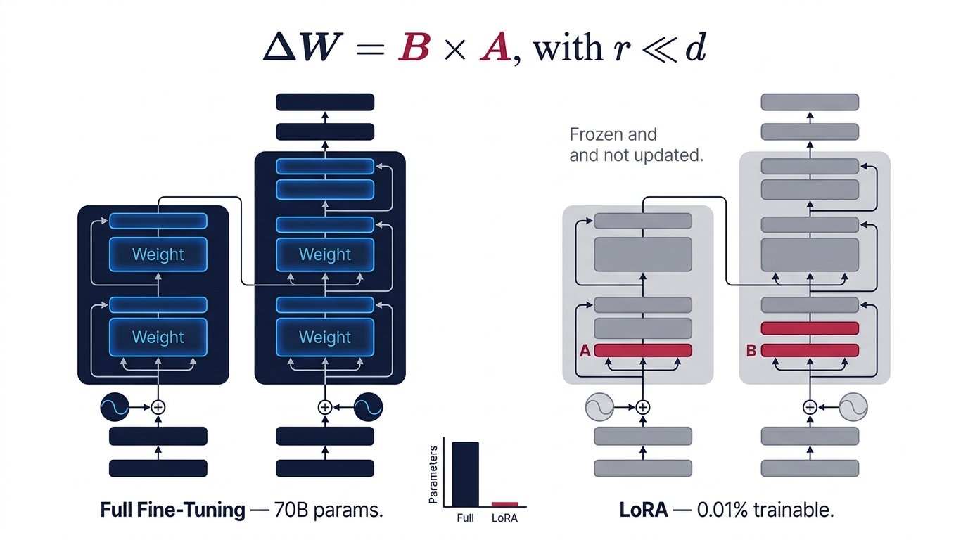
A modern LLM like LLaMA-3 70B contains ~70 billion parameters. Full supervised fine-tuning requires storing the model weights, gradients, and optimizer states (Adam stores two moment vectors per parameter). In fp32 that means roughly 840 GB of GPU memory — far beyond even the largest single-GPU setups.
Full Fine-Tuning
- All ~70B parameters updated each step
- Optimizer states: 2× model size (Adam)
- Multi-hundred GB VRAM requirement
- Risk of catastrophic forgetting
- Separate checkpoint per task (huge storage)
- Impractical on consumer hardware
LoRA Fine-Tuning
- Only adapter matrices trained (~0.1–1% of params)
- Base model weights frozen — no optimizer states for them
- Fits on a single 24 GB GPU for 7B models
- Base knowledge preserved; adapters are modular
- Tiny adapter files (~10–50 MB) per task
- Runs efficiently on consumer GPUs
The Core Mathematics
In a standard transformer layer, a weight matrix W ∈ ℝd×k is updated during fine-tuning as W’ = W + ΔW. Full fine-tuning learns this entire ΔW. LoRA constrains it:
ΔW ∈ ℝd×k → up to d×k trainable params
// LoRA decomposes ΔW into two low-rank matrices
ΔW = B × A
where B ∈ ℝd×r, A ∈ ℝr×k, and r ≪ min(d, k)
// Trainable params: r×d + r×k vs d×k
// For d=4096, k=4096, r=4: ~32K vs ~16.7M
The key insight is rank decomposition: if the true task-adaptation signal lives in a low-dimensional subspace, then ΔW can be well-approximated by a low-rank matrix. Empirically, this holds for a wide range of NLP tasks.
Initialization & Scaling
During training, A is initialized with random Gaussian noise, and B is initialized to all zeros — so ΔW = BA = 0 at the start, meaning the model begins exactly as the pretrained base. The output is scaled by α/r, where α is a tunable hyperparameter:
h = W₀x + ΔWx
h = W₀x + BAx × (α / r)
// W₀ is frozen (no gradient flows through it)
// Only A and B accumulate gradients
// α controls the magnitude of the adaptation
Architecture: What Gets Adapted
Base Model (frozen)
LoRA Adapters (trainable)
Merged Output
Same inference cost
as base model!
LoRA adapters are typically applied to the query and value projection matrices in self-attention (W_Q, W_V). The original paper showed this is often sufficient; many practitioners now also adapt W_K, W_O, and sometimes feed-forward layers.
Choosing the Rank r
The rank r is the single most important hyperparameter. It controls the expressivity–efficiency tradeoff:
Per weight matrix. A 7B model has ~224 such matrices in attention layers.
Practical guidance
For most instruction-following and domain-adaptation tasks, r = 4 to r = 16 works well. Complex reasoning tasks or tasks requiring significant behavioral shifts may benefit from r = 32 or r = 64. Beyond that, you approach full fine-tuning and lose the efficiency benefits without significant quality gain.
PEFT Family: LoRA vs Alternatives
| Method | Trainable Params | Inference Overhead | Key Idea | Best For |
|---|---|---|---|---|
| LoRA | ~0.1–1% | None (merge) | Low-rank ΔW decomposition | General purpose, production |
| QLoRA | ~0.1–1% | +dequant cost | LoRA + 4-bit NormalFloat quantization | Consumer GPU, 65B models on 48GB |
| Prefix Tuning | ~0.1% | +prefix tokens | Prepend trainable prefix tokens | Generation tasks, NLG |
| Prompt Tuning | <0.01% | +soft tokens | Learnable soft prompt embeddings | Very large models (>10B) |
| Adapter Layers | ~0.5–3% | +sequential bottleneck | Small FFN inserted after each layer | Multi-task learning |
| IA³ | <0.1% | Minimal | Scale activations with learned vectors | Few-shot settings |
| DoRA | ~0.1–1% | None (merge) | Decomposes into magnitude + direction | Improved over LoRA on some tasks |
Implementing LoRA in Practice
The Hugging Face PEFT library makes LoRA nearly plug-and-play. Below is a minimal working example for fine-tuning a Mistral-7B model:
from transformers import AutoModelForCausalLM, AutoTokenizer
from peft import LoraConfig, get_peft_model, TaskType

# Load base model (frozen by default in PEFT)
model = AutoModelForCausalLM.from_pretrained(
    "mistralai/Mistral-7B-v0.1",
    device_map="auto",
    torch_dtype=torch.bfloat16,
)

# Define LoRA config
lora_config = LoraConfig(
    task_type=TaskType.CAUSAL_LM,
    r=16,            # rank
    lora_alpha=32,   # scaling: alpha/r = 2.0
    lora_dropout=0.05,
    target_modules=["q_proj", "v_proj", "k_proj", "o_proj"],
)

# Wrap model — only adapter params require grad
model = get_peft_model(model, lora_config)
model.print_trainable_parameters()
# trainable params: 20,971,520 || all params: 7,262,244,864 (0.29%)

# After training, merge and unload for zero-latency inference
model = model.merge_and_unload()
QLoRA: Pushing Further
QLoRA (Dettmers et al., 2023) adds 4-bit quantization of the frozen base model using a new data type called NormalFloat4 (NF4), which is information-theoretically optimal for normally distributed weights. The adapters themselves remain in bf16/fp32. This enables fine-tuning a 65B parameter model on a single 48 GB A100.
Base model weights (NF4): ~32.5 GB
LoRA adapter weights (bf16): ~0.7 GB
Optimizer states (fp32): ~2.1 GB (adapters only)
Activations: ~6.0 GB
Total: ~41.3 GB ← fits in 48GB A100
// vs Full FT in bf16: ~780 GB (≈16× A100s)
Merging & Deployment
One of LoRA’s elegances is that at inference time, the adapter can be merged back into the base weights: W’ = W + BA. The merged model is mathematically identical to a full fine-tuned model with the same ΔW — but was far cheaper to produce. No extra inference latency, no architectural changes.
Alternatively, adapters can be kept separate and hot-swapped at runtime — enabling a single GPU server to host one base model and switch between dozens of specialized task adapters, each ~10–50 MB, with minimal overhead.
Hyperparameter Guide
| Parameter | Typical Range | Effect |
|---|---|---|
r (rank) |
4, 8, 16, 32, 64 | Controls expressivity. Start with 8 or 16. Lower saves memory; higher may improve complex tasks. |
lora_alpha |
16–64 (often 2×r) | Scales adapter outputs by α/r. Higher α amplifies adapter influence. Common heuristic: α = 2r. |
lora_dropout |
0.0–0.1 | Regularization. Use 0.05 for small datasets; 0.0 for large datasets. |
target_modules |
q_proj, v_proj (min); all attention (more) | Which weight matrices to adapt. More modules = more params = better quality at higher cost. |
| Learning rate | 1e-4 to 3e-4 | Higher than full FT is usually safe since adapter weights are small. Use cosine schedule. |